Activity 6: Effect of the temperature#
Surface and bulk effects of the temperature#
In this example, we will look at the effects of the temperature on the X-Ray photoelectron diffraction from a copper substrate. We will base our python script on a paper published in 1986 by R. Trehan and S. Fadley. In their work, they performed azimutal scans of a copper(001) surface at 2 different polar angles: one at grazing incidence and one at 45° for incresing temperatures from 298K to roughly 1000K.
For each azimutal scan, they looked at the anisotropy of the signal, that is:
This value is representative of how clear are the modulations of the signal. They also proposed single scattering calculations that reproduced well these results.
We will reproduce this kind of calculations to introduce the parameters that control the vibrational damping.
See also
based on this paper from R. Trehan and C.S. Fadley Phys. Rev. B 34 p6784–98 (2012)
The script#
Since we want to distinguish between bulk (low polar angles, \(\theta = 45°\) in the paper) and surface effects (large polar angles, \(\theta = 83°\) in the paper), we need to compute scans for different emitters and different depths in the cluster.
The script contains 3 functions:
The
create_clustersfunction will build clusters with increasing number of planes, with the emitter being in the deepest plane for each cluster.The function
computewill compute the azimuthal scan for a given cluster.The
analysisfunction will sum the intensity from each plane for a given temperature. This will be the substrate total signal (more on this in the Activity 7: Large clusters and path filtering section). The function will also compute the anisotropy (equation (1)).
MsSpec can introduce temperature effects in two ways: either by using the Debye Waller model or by doing an average over the phase shifts. We will explore the latter in this example.
Regardless of the option chosen to model temperature effects, we need to define mean square displacement (MSD) values of the atoms in our cluster. We will use the Debye model for this. The MSD is defined as follows:
where \(\hbar\) is the reduce Planck’s constant, \(T\) is the temperature, \(M\) is the mass of the atom, \(k_B\) is the Boltzmann’s constant and \(\Theta_D\) is the Debye temperature of the sample.
To get an idea of the typical order of magnitude for MSD, the figure below plots the values of MSD for copper for temperatures ranging from 300 K to 1000 K.
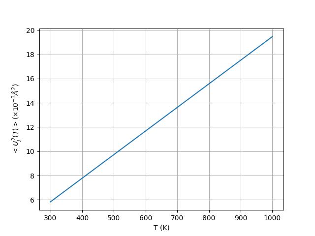
Fig. 14 Variation of MSD for copper versus temperature using equation (2)#
With the help of the MsSpec documentation and the second paragraph p6791 of the article cited above, complete the hilighted lines in the following script to compute the anisotropy of Cu(2p) \(\phi\)-scans for polar angle \(\theta\)=45° and 83°.
How is varying the anisotropy versus the temperature. How can you qualitatively explain this variation ?
  1from ase.build import bulk
  2import numpy as np
  3
  4from msspec.calculator import MSSPEC, XRaySource
  5from msspec.utils import hemispherical_cluster, get_atom_index
  6
  7def create_clusters(nplanes=3):
  8    copper  = bulk('Cu', a=3.6, cubic=True)
  9    clusters = []
 10    for emitter_plane in range(nplanes):
 11        cluster = hemispherical_cluster(copper,
 12                                        emitter_plane=emitter_plane,
 13                                        planes=emitter_plane+1,
 14                                        diameter=27,
 15                                        shape='cylindrical')
 16        cluster.absorber = get_atom_index(cluster, 0, 0, 0)
 17        # This is how to store extra information with your cluster
 18        cluster.info.update({
 19            'emitter_plane': emitter_plane,
 20        })
 21        clusters.append(cluster)
 22    return clusters
 23
 24
 25def compute(clusters, all_theta=[45., 83.],
 26            all_T=np.arange(300., 1000., 400.)):
 27    data = None
 28    for cluster in clusters:
 29        # Retrieve emitter's plane from cluster object
 30        plane   = cluster.info['emitter_plane']
 31
 32        calc = MSSPEC(spectroscopy='PED', algorithm='expansion')
 33        calc.source_parameters.energy = XRaySource.AL_KALPHA
 34        calc.muffintin_parameters.interstitial_potential = 14.1
 35
 36        # In simple scattering, it is common practice to use a real potential and
 37        # manually define a mean free path arbitrarily lower than the actual physical
 38        # value in an attempt to reproduce multiple scattering effects.
 39        calc.tmatrix_parameters.exchange_correlation = 'x_alpha_real'
 40        calc.calculation_parameters.mean_free_path = ... # -> half of the mean free
 41                                                         # path (see p6785)
 42        # Parameters for temperature effects
 43        calc.calculation_parameters.vibrational_damping = 'averaged_tl'
 44        calc.calculation_parameters.use_debye_model = ..... # Use the MsSpec help
 45        calc.calculation_parameters.debye_temperature = ... # and p6791 of the paper
 46        calc.calculation_parameters.vibration_scaling = ... # -> How much more do
 47                                                            # surface atoms vibrate
 48                                                            # than bulk atoms?
 49        calc.detector_parameters.average_sampling = 'low'
 50        calc.detector_parameters.angular_acceptance = 5.7
 51
 52        calc.calculation_parameters.scattering_order = 1
 53
 54
 55        for T in all_T:
 56            # Define the sample temperature
 57            calc.calculation_parameters.temperature = T
 58            # Set the atoms and compute an azimuthal scan
 59            calc.set_atoms(cluster)
 60            data = calc.get_phi_scan(level='2p', theta=all_theta,
 61                                        phi=np.linspace(0, 100, 51),
 62                                        kinetic_energy=560, data=data)
 63            # Small changes to add some details in both the title of the dataset
 64            # and the figure
 65            view = data[-1].views[-1]
 66            t = view._plotopts['title'] + f" (plane #{plane:d}, T={T:.0f} K)"
 67            data[-1].title = t
 68            view.set_plot_options(autoscale=True, title=t)
 69        calc.shutdown()
 70    return data
 71
 72
 73def analysis(data, all_theta, all_T, nplanes):
 74    # Sum cross_section for all emitter's plane at a given T
 75    # Compute the anisotropy
 76    results = dict.fromkeys(all_T, [])
 77    anisotropy = []
 78    for dset in data:
 79        # Retrieve temperature
 80        T = float(dset.get_parameter('CalculationParameters', 'temperature')['value'])
 81        # Update the sum in results
 82        if len(results[T]) == 0:
 83            results[T] = dset.cross_section
 84        else:
 85            results[T] += dset.cross_section
 86
 87    anisotropy_dset = data.add_dset("Anisotropies")
 88    anisotropy_dset.add_columns(temperature=all_T)
 89    for theta in all_theta:
 90        col_name = f"theta{theta:.0f}"
 91        col_values = []
 92        i = np.where(dset.theta == theta)[0]
 93        for T in all_T:
 94            cs = results[T][i]
 95            Imax = np.max(cs)
 96            Imin = np.min(cs)
 97            A = (Imax - Imin)/Imax
 98            col_values.append(A)
 99        anisotropy_dset.add_columns(**{col_name:col_values/np.max(col_values)})
100
101
102    anisotropy_view = anisotropy_dset.add_view('Anisotropies',
103                         title='Relative anisotropies for Cu(2p)',
104                         marker='o',
105                         xlabel='T (K)',
106                         ylabel=r'$\frac{\Delta I / I_{max}(T)}{\Delta I_{300}'
107                                r'/ I_{max}(300)} (\%)$',
108                         autoscale=True)
109    for theta in all_theta:
110        col_name = f"theta{theta:.0f}"
111        anisotropy_view.select('temperature', col_name,
112                                legend=r'$\theta = {:.0f} \degree$'.format(theta))
113
114    return data
115
116
117
118if __name__ == "__main__":
119    nplanes = 4
120    all_theta = np.array([45, 83])
121    all_theta = np.array([300., 1000.])
122
123    clusters = create_clusters(nplanes=nplanes)
124    data = compute(clusters, all_T=all_T, all_theta=all_theta)
125    data = analysis(data, all_T=all_T, all_theta=all_theta, nplanes=nplanes)
126    data.view()
  1from ase.build import bulk
  2import numpy as np
  3
  4from msspec.calculator import MSSPEC, XRaySource
  5from msspec.utils import hemispherical_cluster, get_atom_index
  6
  7def create_clusters(nplanes=3):
  8    copper  = bulk('Cu', a=3.6, cubic=True)
  9    clusters = []
 10    for emitter_plane in range(nplanes):
 11        cluster = hemispherical_cluster(copper,
 12                                        emitter_plane=emitter_plane,
 13                                        planes=emitter_plane+1,
 14                                        diameter=27,
 15                                        shape='cylindrical')
 16        cluster.absorber = get_atom_index(cluster, 0, 0, 0)
 17        # This is how to store extra information with your cluster
 18        cluster.info.update({
 19            'emitter_plane': emitter_plane,
 20        })
 21        clusters.append(cluster)
 22    return clusters
 23
 24
 25def compute(clusters, all_theta=[45., 83.],
 26            all_T=np.arange(300., 1000., 400.)):
 27    data = None
 28    for cluster in clusters:
 29        # Retrieve emitter's plane from cluster object
 30        plane   = cluster.info['emitter_plane']
 31
 32        calc = MSSPEC(spectroscopy='PED', algorithm='expansion')
 33        calc.source_parameters.energy = XRaySource.AL_KALPHA
 34        calc.muffintin_parameters.interstitial_potential = 14.1
 35
 36        # In simple scattering, it is common practice to use a real potential and
 37        # manually define a mean free path arbitrarily lower than the actual physical
 38        # value in an attempt to reproduce multiple scattering effects.
 39        calc.tmatrix_parameters.exchange_correlation = 'x_alpha_real'
 40        calc.calculation_parameters.mean_free_path = .5 * 9.1
 41
 42        # Parameters for temperature effects
 43        calc.calculation_parameters.vibrational_damping = 'averaged_tl'
 44        calc.calculation_parameters.use_debye_model = True
 45        calc.calculation_parameters.debye_temperature = 343
 46        calc.calculation_parameters.vibration_scaling = 2.3
 47
 48
 49        calc.detector_parameters.average_sampling = 'low'
 50        calc.detector_parameters.angular_acceptance = 5.7
 51
 52        calc.calculation_parameters.scattering_order = 1
 53
 54
 55        for T in all_T:
 56            # Define the sample temperature
 57            calc.calculation_parameters.temperature = T
 58            # Set the atoms and compute an azimuthal scan
 59            calc.set_atoms(cluster)
 60            data = calc.get_phi_scan(level='2p', theta=all_theta,
 61                                        phi=np.linspace(0, 100, 51),
 62                                        kinetic_energy=560, data=data)
 63            # Small changes to add some details in both the title of the dataset
 64            # and the figure
 65            view = data[-1].views[-1]
 66            t = view._plotopts['title'] + f" (plane #{plane:d}, T={T:.0f} K)"
 67            data[-1].title = t
 68            view.set_plot_options(autoscale=True, title=t)
 69        calc.shutdown()
 70    return data
 71
 72
 73def analysis(data, all_theta, all_T, nplanes):
 74    # Sum cross_section for all emitter's plane at a given T
 75    # Compute the anisotropy
 76    results = dict.fromkeys(all_T, [])
 77    anisotropy = []
 78    for dset in data:
 79        # Retrieve temperature
 80        T = float(dset.get_parameter('CalculationParameters', 'temperature')['value'])
 81        # Update the sum in results
 82        if len(results[T]) == 0:
 83            results[T] = dset.cross_section
 84        else:
 85            results[T] += dset.cross_section
 86
 87    anisotropy_dset = data.add_dset("Anisotropies")
 88    anisotropy_dset.add_columns(temperature=all_T)
 89    for theta in all_theta:
 90        col_name = f"theta{theta:.0f}"
 91        col_values = []
 92        i = np.where(dset.theta == theta)[0]
 93        for T in all_T:
 94            cs = results[T][i]
 95            Imax = np.max(cs)
 96            Imin = np.min(cs)
 97            A = (Imax - Imin)/Imax
 98            col_values.append(A)
 99        anisotropy_dset.add_columns(**{col_name:col_values/np.max(col_values)})
100
101
102    anisotropy_view = anisotropy_dset.add_view('Anisotropies',
103                         title='Relative anisotropies for Cu(2p)',
104                         marker='o',
105                         xlabel='T (K)',
106                         ylabel=r'$\frac{\Delta I / I_{max}(T)}{\Delta I_{300}'
107                                r'/ I_{max}(300)} (\%)$',
108                         autoscale=True)
109    for theta in all_theta:
110        col_name = f"theta{theta:.0f}"
111        anisotropy_view.select('temperature', col_name,
112                                legend=r'$\theta = {:.0f} \degree$'.format(theta))
113
114    return data
115
116
117
118if __name__ == "__main__":
119    nplanes = 4
120    all_theta = np.array([45, 83])
121    all_theta = np.array([300., 1000.])
122
123    clusters = create_clusters(nplanes=nplanes)
124    data = compute(clusters, all_T=all_T, all_theta=all_theta)
125    data = analysis(data, all_T=all_T, all_theta=all_theta, nplanes=nplanes)
126    data.view()
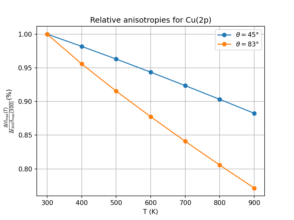
Fig. 15 Variation of anisotropy as a function of temperature and polar angle for Cu(2p).#
The anisotropy decreases when the temperature is increased due to the increased disorder in the structure coming from thermal agitation. This variation in anisotropy is more pronounced for grazing incidence angles since surface atoms are expected to vibrate more than bulk ones and the expected mean depth of no-loss emission is \(\sim 1\) atomic layer at \(\theta = 83°\) and 3-4 layers at \(\theta = 45°\) as estimated by \(\Lambda_e\sin\theta\) (where \(\Lambda_e\) is the photoelectron mean free path at 560 eV).