Activity 4: From single scattering to multiple scattering

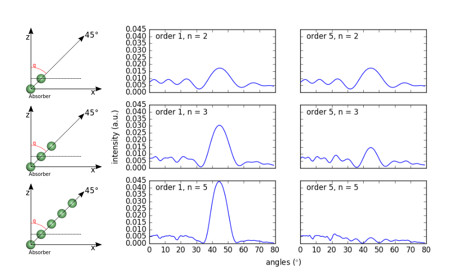
Fig. 10 Polar scan of a Ni chain of 2-5 atoms for single and mutliple (5^th order) scattering.

See also

based on this paper from M.-L. Xu et al. Phys. Rev. B 39 p8275 (1989)

# coding: utf-8

# import all we need and start by msspec
from msspec.calculator import MSSPEC

# we will build a simple atomic chain
from ase  import Atom, Atoms

# we need some numpy functions
import numpy as np


symbol = 'Ni'            # The kind of atom for the chain
orders = (1, 5)          # We will run the calculation for single scattering
                         # and multiple scattering (5th diffusion order)
chain_lengths = (2,3,5)  # We will run the calculation for differnt lengths
                         # of the atomic chain
a = 3.499 * np.sqrt(2)/2 # The distance bewteen 2 atoms

# Define an empty variable to store all the results
all_data = None

# 2 for nested loops over the chain length and the order of diffusion
for chain_length in chain_lengths:
    for order in orders:
        # We build the atomic chain by
        #    1- stacking each atom one by one along the z axis
        chain = Atoms([Atom(symbol, position = (0., 0., i*a)) for i in
                       range(chain_length)])
        #    2- rotating the chain by 45 degrees with respect to the y axis
        #chain.rotate('y', np.radians(45.))
        chain.rotate(45., 'y')
        #    3- setting a custom Muffin-tin radius of 1.5 angstroms for all
        #       atoms (needed if you want to enlarge the distance between
        #       the atoms while keeping the radius constant)
        #[atom.set('mt_radius', 1.5) for atom in chain]
        #    4- defining the absorber to be the first atom in the chain at
        #       x = y = z = 0
        chain.absorber = 0

        # We define a new PED calculator
        calc = MSSPEC(spectroscopy = 'PED')
        calc.set_atoms(chain)
        # Here is how to tweak the scattering order
        calc.calculation_parameters.scattering_order = order
        # This line below is where we actually run the calculation
        all_data = calc.get_theta_scan(level='3s', #kinetic_energy=1000.,
                            theta=np.arange(0., 80.), data=all_data)

        # OPTIONAL, to improve the display of the data we will change the dataset
        # default title as well as the plot title
        t = "order {:d}, n = {:d}".format(order, chain_length) # A useful title
        dset = all_data[-1]         # get the last dataset
        dset.title = t              # change its title
        # get its last view (there is only one defined for each dataset)
        v = dset.views()[-1]
        v.set_plot_options(title=t) # change the title of the figure



# OPTIONAL, set the same scale for all plots
# 1. iterate over all computed cross_sections to find the absolute minimum and
# maximum of the data
min_cs = max_cs = 0
for dset in all_data:
    min_cs = min(min_cs, np.min(dset.cross_section))
    max_cs = max(max_cs, np.max(dset.cross_section))

# 2. for each view in each dataset, change the scale accordingly
for dset in all_data:
    v = dset.views()[-1]
    v.set_plot_options(ylim=[min_cs, max_cs])

# Pop up the graphical window
all_data.view()
# You can end your script with the line below to remove the temporary
# folder needed for the calculation
calc.shutdown()

Quiz

Some questions to answer