Activity 2: Setting up the “experiment”

To model a spectroscopy experiment, some parameters need to be correctly defined. In MsSpec, parameters are grouped in different categories (detector_parameters, source_parameters, calculation_parameters…). Each category is an attribute of your calculator object and contains different parameters. For example, to define the angle of the incoming light with respect to the sample normal direction, you will use

# (assuming your calculator variable is calc)
# e.g: Incoming X-Ray light is 30° from the sample normal
calc.source_parameters.theta = 30

Sb-induced smooth growth of Ag on Ag(111) example

To see how some parameters - not related to the cluster shape - may change the results, we will look at the effect of two parameters:

1. The source direction

2. The inner potential of the sample

The inner potential is material specific. It will add to the photoelectron kinetic energy inside the material. When the photoelectron escapes the sample, this internal potential is missing and this will create an energy step that will act as a refraction for the photoelectron intensity. The effect will be significant for large polar angles and for small kinetic energy of the photoelectron.

Let’s look at the effect of those parameters on the following example. The idea is to use low energy photoelectron diffraction to see the substitution of Ag by Sb atoms on the surface plane.

See also

based on this paper from H. Cruguel et al. Phys. Rev. B 55 R16061

Building the cluster

Let’s start by building the cluster

from ase.build import bulk
from ase.visualize import view

from msspec.calculator import MSSPEC
from msspec.utils import hemispherical_cluster, get_atom_index, cut_plane
import numpy as np
from matplotlib import pyplot as plt

# Create the silver cell
Ag = bulk('Ag', cubic=True)
# Orientate the cell in the [111] direction
Ag.rotate((1,1,1), (0,0,1), rotate_cell=True)
# Align the azimuth to match experimental reference
Ag.rotate(15, 'z', rotate_cell=True)

# Create a cluster
cluster = hemispherical_cluster(Ag, diameter=20, emitter_plane=0)
cluster = cut_plane(cluster, z=-4.8)
cluster.emitter = get_atom_index(cluster, 0,0,0)
cluster[cluster.emitter].symbol = 'Sb'

Compute an azimuthal scan

Now create a calculator and configure experimental parameters

# Define parameters
calc.source_parameters.theta = 0
calc.source_parameters.phi = 0

calc.detector_parameters.angular_acceptance = 1
calc.detector_parameters.average_sampling = 'low'

calc.muffintin_parameters.interstitial_potential = 0

Finally, add those lines to compute the \(\phi\)-scan (in orange) and compare it to the experimental data (in blue).

# Compute an azimuthal scan
data = calc.get_phi_scan(level='4d', theta=40, phi=np.linspace(0,240,121), kinetic_energy=45)

# Normalize data between [0,1] (to ease comparison with experimental data)
dset = data[0]
dset.cross_section -= dset.cross_section.min()
dset.cross_section /= dset.cross_section.max()

# Add experimental data points in the dataset
x, y = np.loadtxt('data.txt').T
dset.add_columns(experiment=y)

# Add points to view
view = dset.views[0]
view.select('phi', 'experiment', legend='Exp. data')

# Popup GUI
data.view()

# Remove temp. files
calc.shutdown()

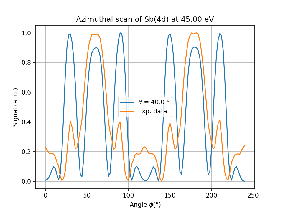
Fig. 4 Azimuthal (\(\phi\)) scan for Sb(4d) emitter in the top layer of Ag(111) at 45 eV kinetic energy.

The agreement is not satisfactory although most of the features may be identified.

Quiz

Try to change the source direction and the inner potential of Ag to better match the experiment…

Note

The cluster is smaller than it should for size convergence, but the calculation would take too much memory for this example

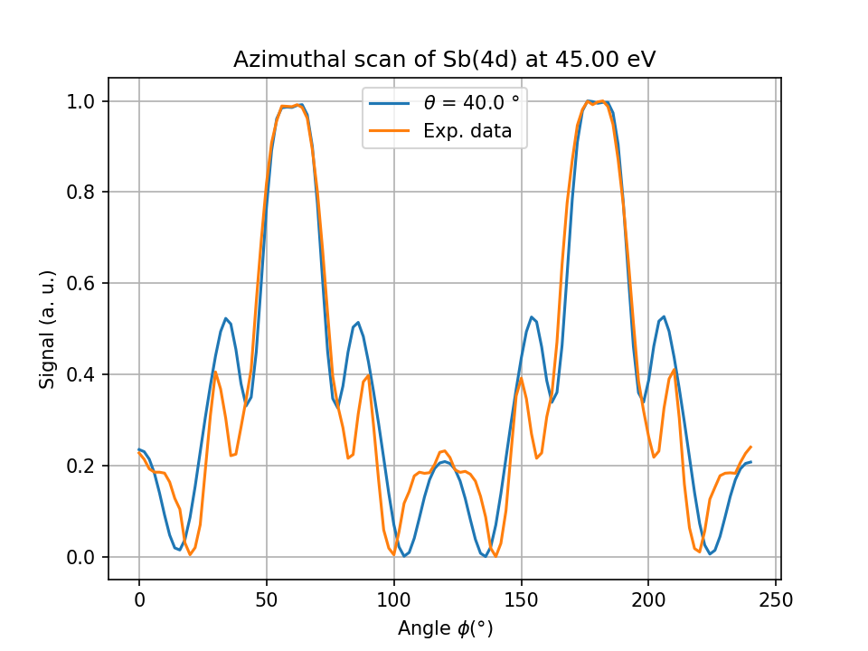
Fig. 5 Azimuthal (\(\phi\)) scan for Sb(4d) emitter in the top layer of Ag(111) at 45 eV kinetic energy, with muffintin_parameters.interstitial_potential = 10.2 and source_parameters.theta = 22.5

# Source geometry (the former SA73 beamline of the LURE synchrotron)
# given in ref 6 of the paper...
calc.source_parameters.theta = 22.5
# Inner potential is generally between 10 and 20 eV for most metrials
calc.muffintin_parameters.inner_potential = 10.2