Activity 8: Inequivalent emitters and the XPD of a substrate#
XPD can be used to study the adsorption of atoms or molecules on surfaces (Activity 3), or atomic substitutions on surfaces (Activity 2). In this case, modeling is relatively straightforward, since only one emitter atom is involved.
We have seen from previous examples that, for kinetic energies \(\gtrsim\) 500 eV, the use of Rehr-Albers series expansion and scattering path filtering give access to the intensity of deeper emitter atoms (Activity 7). This is the key to computing the total photodiffraction signal of a substrate. As emitted photoelectrons originate from highly localized core levels around the atoms, the total signal corresponds to the (incoherent) sum of the intensities of all inequivalent emitters in the probed volume.
Let’s take a look at how this is done on the following example.
The Aluminium Nitride (AlN) polarity#
In this example, we will compute polar diagrams of an aluminum nitride substrate.
In a work published in 1999, Lebedev et al. demonstrated that Photoelectron diffraction can be used as a non invasive tool to unambiguously state the polarity of an AlN surface. Aluminium nitride cristallizes in an hexagonal cell and the authors experimentally showed that the polarity of the surface can be controlled by the annealing temperature during the growth. Both polarities are sketched in the figure below.
See also
based on this paper from V. Lebedev et al. J. Cryst. Growth. 207(4) p266-72 (1999)
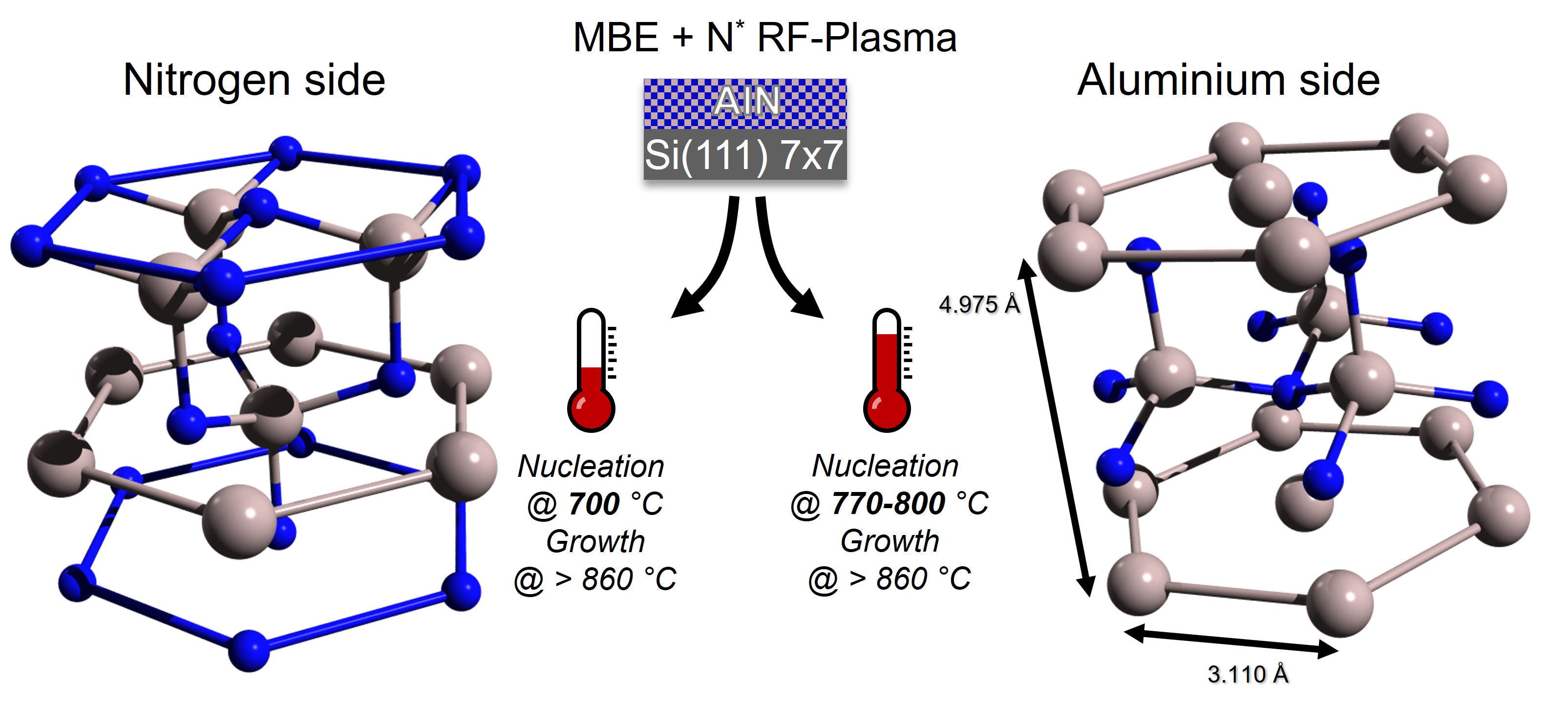
Fig. 21 AlN hexagonal lattice. Left) N polarity with nitrogen terminated surface and AlN4 tetrahedrons pointing downward. Right) Al polarity with aluminium terminated surface and AlN4 tetrahedrons pointing upward#
The AlN(0001) and (00.-1) faces share the same crystallograpphic symmetry and the Al and N atoms have the same geometrical surrounding differing only in the exchange of Al and N atoms (Fig. 22).
It is thus expected that Al(2p) and N(1s) XPD patterns exhibit almost the same features with only small differences due to the contrast between Al and N scattering amplitudes.
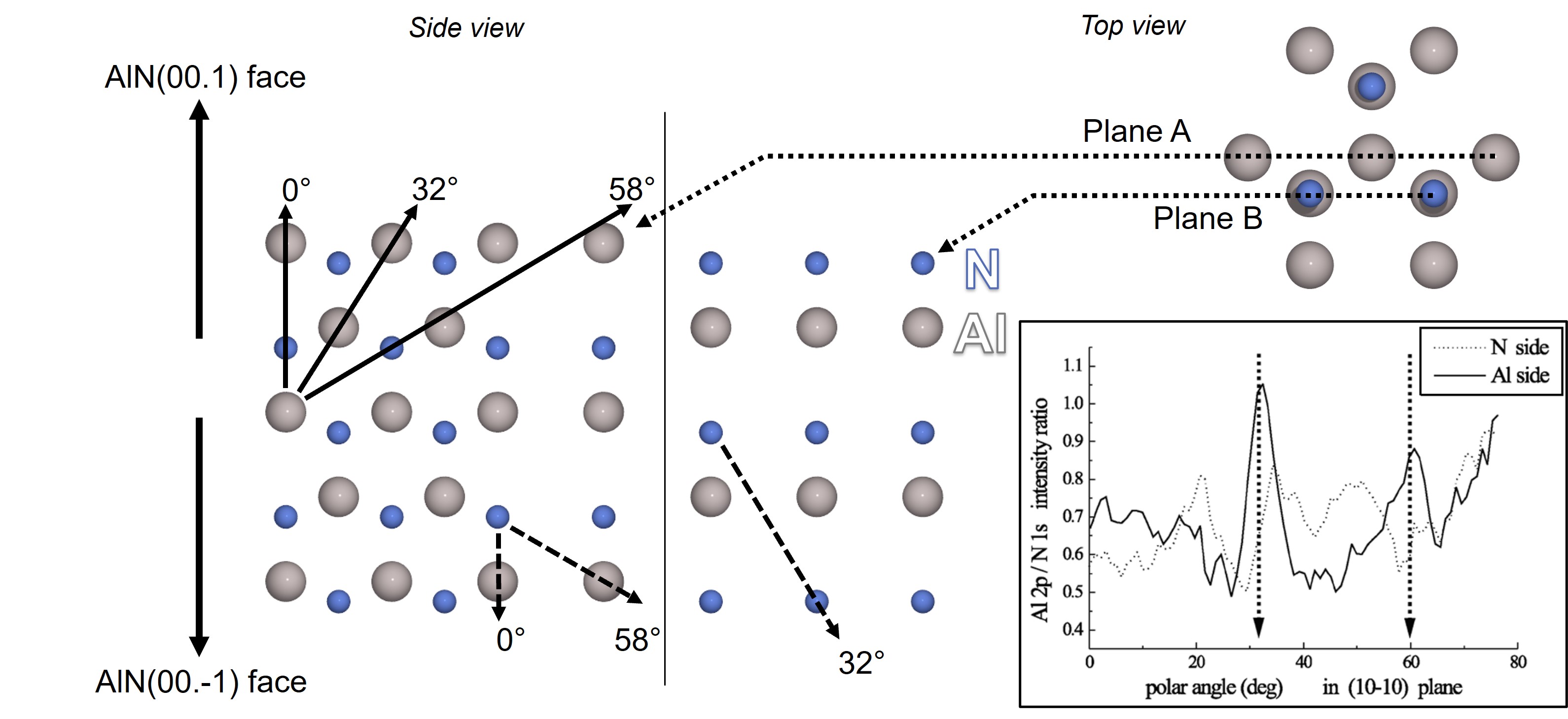
Fig. 22 Side views of N- or Al- terminated surfaces showing nearest neighbours main polar crystallographic directions. The inset shows the experimental Al(2p)/N(1s) ratio versus polar angle for both AlN polarities (taken from Lebedev et al.).#
The strongest differences in photoemission intensities suitable for a quick and unambiguous determination of polarity were found in the (10-10) azimuthal plane at 32° and 59° (polar scans in the inset of Fig. 22).
These are the directions of short neighbor distances between the atoms of the same element (32°) and between Al and N atoms (58.5°), respectively.
Using the crystal view in Fig. 21 and assuming that we want to compute Al(2p) and N(1s) intensities for emitters located in 3 different planes to get a substrate signal. How many clusters do we need to build ?
Solution…
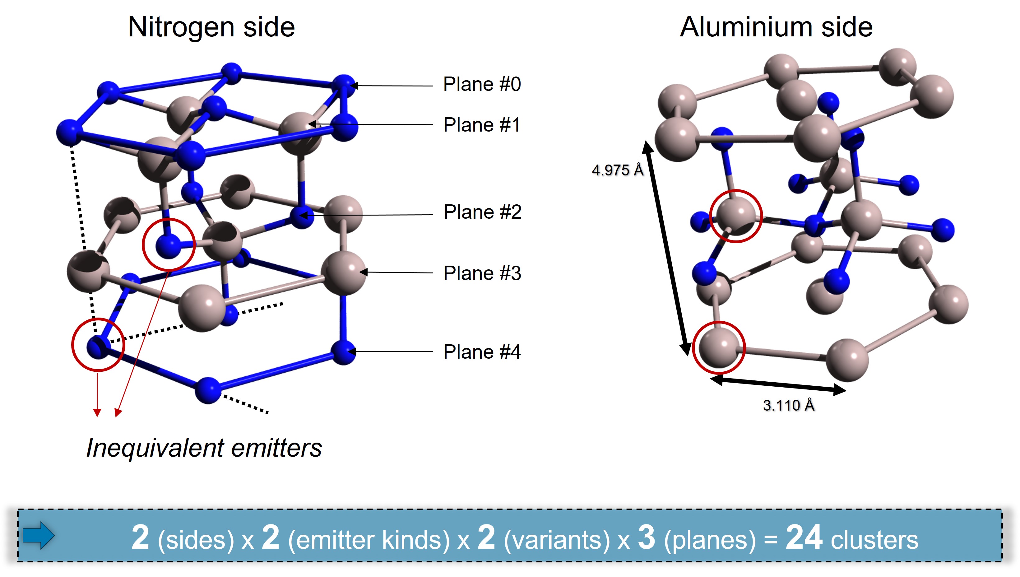
Fig. 23 Number of different clusters to build for Al(2p) and N(1s) in 3 planes#
Download this script and fill in the lines indicated by the comments “FILL HERE”. Run the calculation and check that you are reproducing polar scan of Fig. 22.
Solution…
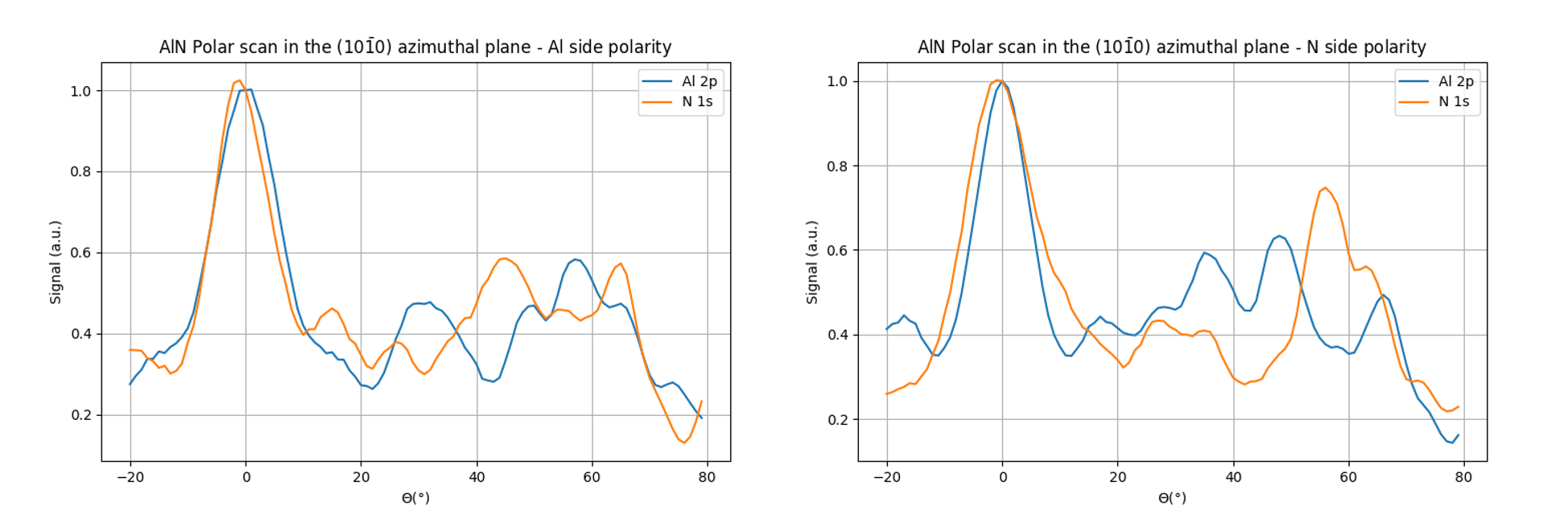
Fig. 24 Polar scans in the (10-10) azimuthal plane of AlN for Al polarity (left) and N polarity (right)#
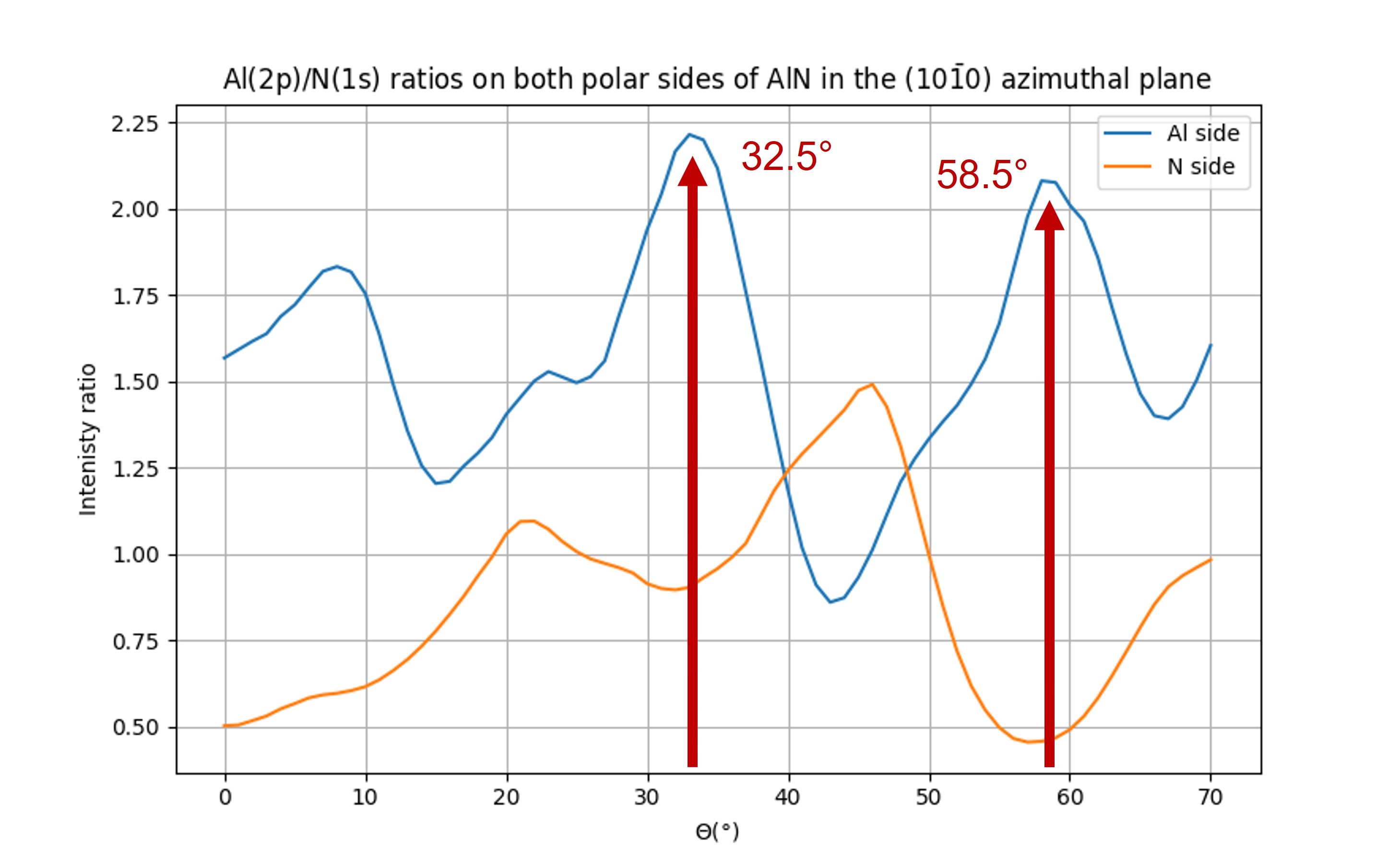
Fig. 25 Al(2p)/N(1s) intensity ratio for both polarities#
As can be seen in Fig. 25, the peaks at 32° and 58.5° are well reproduced by the calculation for an Al polarity. Some discreapancies arise between the experimental work and this simulation especially for large polar angles. This may be due to a too small cluster in diameter for the deeper emitters.
  1from ase.build import bulk
  2import numpy as np
  3from msspec.calculator import MSSPEC, XRaySource
  4from msspec.utils import hemispherical_cluster, get_atom_index
  5
  6def create_clusters(nplanes=6):
  7    def get_AlN_tags_planes(side, emitter):
  8        AlN = bulk('AlN', crystalstructure='wurtzite', a=3.11, c=4.975)
  9        [atom.set('tag', i) for i, atom in enumerate(AlN)]
 10        if side == 'Al':
 11            AlN.rotate([0,0,1],[0,0,-1])
 12            Al_planes = range(0, nplanes, 2)
 13            N_planes  = range(1, nplanes, 2)
 14        else:
 15            N_planes  = range(0, nplanes, 2)
 16            Al_planes = range(1, nplanes, 2)
 17        if emitter == 'Al':
 18            tags = [0, 2]
 19            planes = Al_planes
 20        else:
 21           tags = [1, 3]
 22           planes = N_planes
 23        return AlN, tags, planes
 24
 25    clusters = []
 26    for side in ('Al', 'N'):
 27        for emitter in ('Al', 'N'):
 28            AlN, tags, planes = get_AlN_tags_planes(side, emitter)
 29            for emitter_tag in tags:
 30                for emitter_plane in planes:
 31                    cluster = hemispherical_cluster(AlN,
 32                                                    emitter_tag=emitter_tag,
 33                                                    emitter_plane=emitter_plane,
 34                                                    planes=emitter_plane+2)
 35                    cluster.absorber = get_atom_index(cluster, 0, 0, 0)
 36                    cluster.info.update({
 37                        'emitter_plane': emitter_plane,
 38                        'emitter_tag'  : emitter_tag,
 39                        'emitter'      : emitter,
 40                        'side'         : side,
 41                    })
 42                    clusters.append(cluster)
 43                    print("Added cluster {}-side, emitter {}(tag {:d}) in "
 44                          "plane #{:d}".format(side, emitter, emitter_tag,
 45                                               emitter_plane))
 46    return clusters
 47
 48
 49def compute(clusters, theta=np.arange(-20., 80., 1.), phi=0.):
 50    data = None
 51    for ic, cluster in enumerate(clusters):
 52        # Retrieve info from cluster object
 53        side    = cluster.info['side']
 54        emitter = cluster.info['emitter']
 55        plane   = cluster.info['emitter_plane']
 56        tag     = cluster.info['emitter_tag']
 57
 58        # Set the level and the kinetic energy
 59        if emitter == 'Al':
 60            level = '2p'
 61            ke    = 1407.
 62        elif emitter == 'N':
 63            level = '1s'
 64            ke    = 1083.
 65
 66        calc = MSSPEC(spectroscopy='PED', algorithm='expansion')
 67
 68        calc.source_parameters.energy = XRaySource.AL_KALPHA
 69        calc.source_parameters.theta  = -35
 70
 71        calc.detector_parameters.angular_acceptance = 4.
 72        calc.detector_parameters.average_sampling   = 'medium'
 73
 74        calc.calculation_parameters.scattering_order = max(1, min(4, plane))
 75        calc.calculation_parameters.path_filtering  = 'forward_scattering'
 76        calc.calculation_parameters.off_cone_events = 1
 77        [a.set('forward_angle', 30.) for a in cluster]
 78
 79        calc.set_atoms(cluster)
 80
 81        data = calc.get_theta_scan(level=level, theta=theta, phi=phi,
 82                                   kinetic_energy=ke, data=data)
 83        dset = data[-1]
 84        dset.title = "\'{}\' side - {}({}) tag #{:d}, plane #{:d}".format(
 85            side, emitter, level, tag, plane)
 86
 87    return data
 88
 89
 90def analysis(data):
 91    tmp_data = {}
 92    for dset in data:
 93        info = dset.get_cluster().info
 94        side = info['side']
 95        emitter = info['emitter']
 96        try:
 97            key = '{}_{}'.format(side, emitter)
 98            tmp_data[key] += dset.cross_section
 99        except KeyError:
100            tmp_data[key] = dset.cross_section.copy()
101
102    tmp_data['theta']   = dset.theta.copy()
103    tmp_data['Al_side'] = tmp_data['Al_Al'] / tmp_data['Al_N']
104    tmp_data['N_side']  = tmp_data['N_Al']  / tmp_data['N_N']
105
106    # now add all columns
107    substrate_dset = data.add_dset('Total substrate signal')
108    substrate_dset.add_columns(**tmp_data)
109
110    view = substrate_dset.add_view('Ratios',
111                                   title=r'Al(2p)/N(1s) ratios on both polar '
112                                         r'sides of AlN in the (10$\bar{1}$0) '
113                                         r'azimuthal plane',
114                                   xlabel=r'$\Theta (\degree$)',
115                                   ylabel='Intenisty ratio')
116    view.select('theta', 'Al_side', legend='Al side',
117                where="theta >= 0 and theta <=70")
118    view.select('theta', 'N_side', legend='N side',
119                where="theta >= 0 and theta <=70")
120    view.set_plot_options(autoscale=True)
121
122    return data
123
124
125clusters = create_clusters()
126for cluster in clusters:
127    cluster.edit()
128exit()
129data     = compute(clusters)
130data     = analysis(data)
131data.view()
132