Activity 7: Large clusters and path filtering#
So far you have seen that multiple scattering calculations with MsSpec can use two different algorithms: matrix inversion or Rehr Albers series expansion. When matrix inversion becomes impossible because the kinetic energy is too high and the number of atoms is too large, serial expansion is the alternative. This algorithm requires very little memory but it processes the scattering paths sequentially, which can lead to very long calculation times.
In this activity, we will explore how to configure MsSpec to reduce this calculation time to compute the signal from a deep emitter in Si(001).
The number of scattering paths#
To fix the idea, we will first evaluate how many scattering paths we need to compute for an emitter in the subsurface (2nd plane) or in the bulk (7th plane) of a Si(001) cluster.
Create a cluster of Si(001) with the emitter in the subsurface, 40 Å diameter with 2 planes (since atoms below the emitter can be ignored at high kinetic energies).
For an emitter in the subsurface, we can use single scattering (see Activity 5: Multiple scattering in the forward scattering regime). How many paths would be generated for this calculation ?
Same question for an emitter in the 7th plane. If we were able to treat each scattering path within only 1 µs. How long would be such calculation ?
Note
Remember that
for an emitter in plane \(p\), the scattering order has to be at least the number of planes
abovethe emitterThe number of scattering paths of order \(n\) corresponds to the number of possibilities of arranging up to \(n\) atoms (taking order into account).
To get the total number of paths generated by a cluster of \(N\) atoms up to order \(M\), use the following formula:
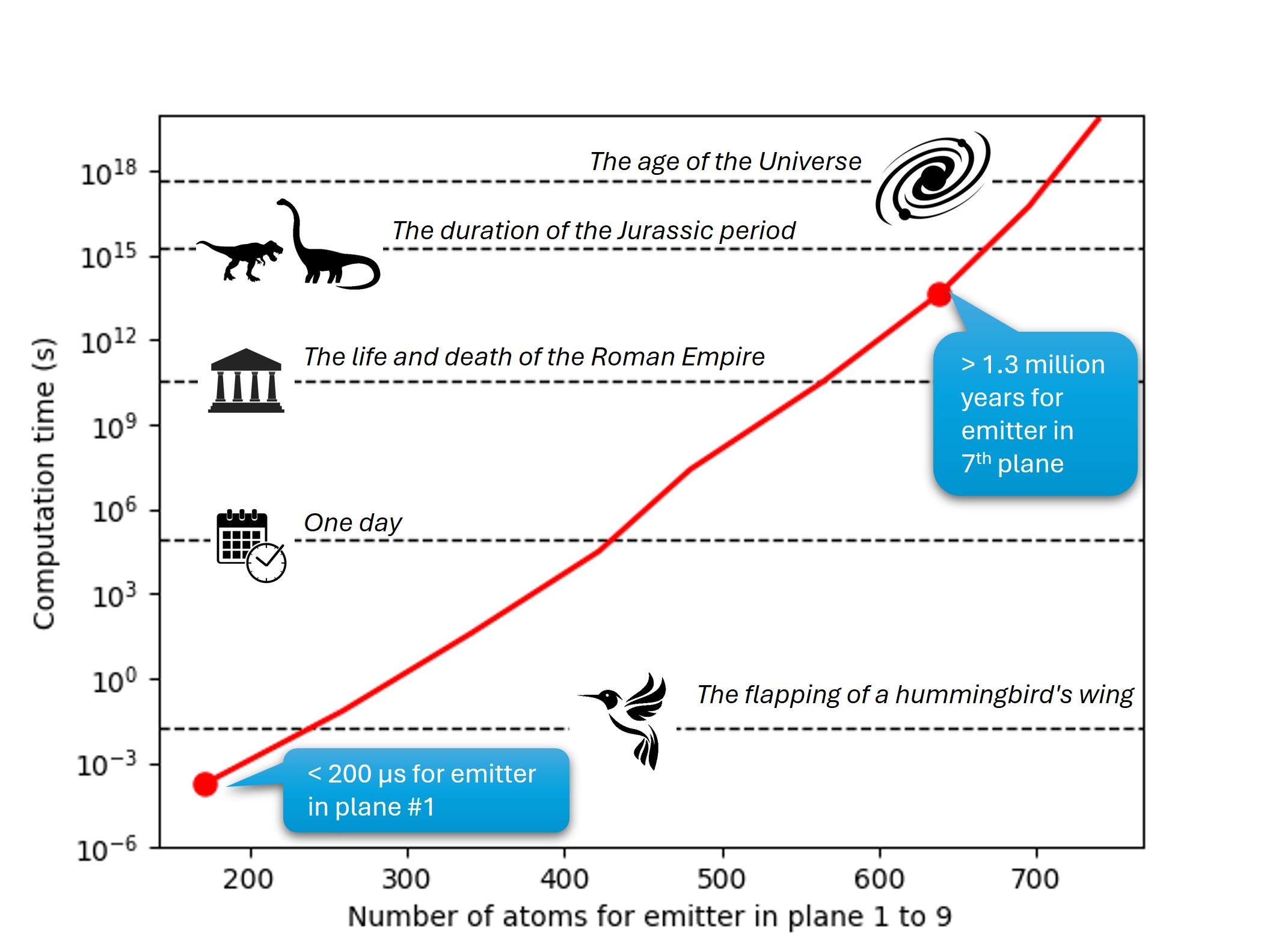
Fig. 16 The time for computing all scattering path for increasing cluster size and scattering order (up to 6th order with 739 atoms. (One path is assumed to be calculated within 1 µs)#
Paths filtering in MsSpec#
As you may expect, not all paths contribute significantly to the total intensity. This is why we can filter out some scattering paths and drastically reduce the computation time. MsSpec offers several filters for this. The 3 most common filters are:
the
forward_scatteringfilter which allows all paths where each scattering angle is within a cone of defined aperturethe
backward_scatteringfilter which is similar to the previous one but for backscattering directionthe
distancefilter which rejects all paths longer than a threshold distance
The following figure illustrate the effect of theses filters on scattering paths
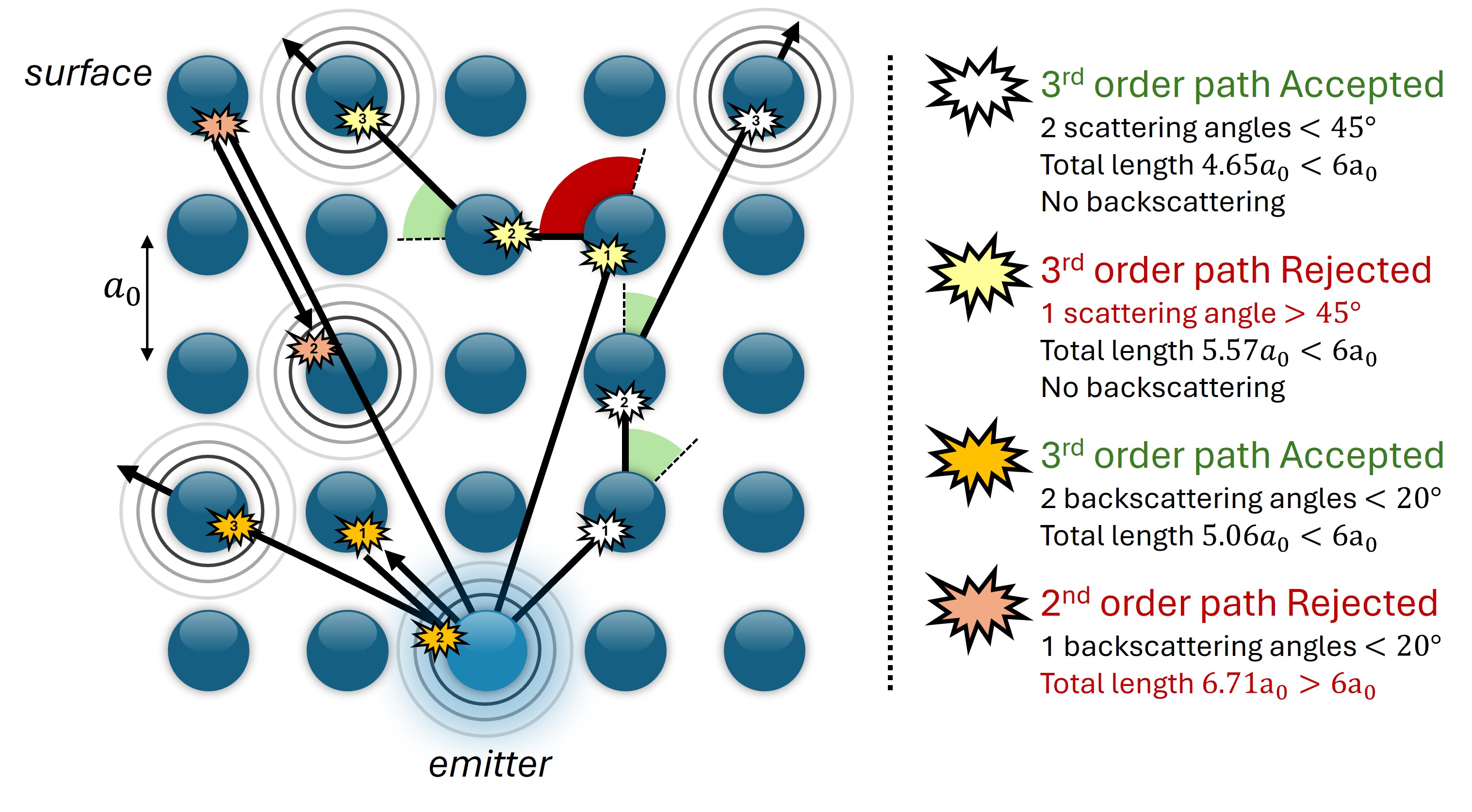
Fig. 17 Some examples of scattering paths with forward_scattering, backward_scattering and distance filters selected. The accepted forward angle is 45°, the accepted backscattering angle is 20° and the threshold distance is \(6a_0\) where \(a_0\) is the lattice parameter. Note that the yellow path is rejected but if the off_cone_events option is set to a value > 1, then it could have been accepted.#
Application to a deep plane in a Si(001) sample#
The following script will compute the contribution of a Si(2p) atom in the 4th plane of a Si(001) cluster at scattering order 3.
Taking into account all scattering paths took 15 minutes to compute.
See also
based on this paper from S. Tricot et al. J. Electron. Spectrosc. Relat. Phenom. 256 147176 (2022)
The following script is almost completed, try to define path filtering options (no backscattering, accept all paths with forward angles < 40° and reject paths longer than the diameter of the cluster).
 1# coding: utf8
 2
 3import numpy as np
 4from ase.build import bulk
 5
 6from msspec.calculator import MSSPEC, XRaySource
 7from msspec.iodata import Data
 8from msspec.utils import hemispherical_cluster, get_atom_index
 9
10
11# Create the cluster
12a = 5.43
13Si = bulk('Si', a=a, cubic=True)
14cluster = hemispherical_cluster(Si,
15                                diameter=30, planes=4,
16                                emitter_plane=3,
17                                shape = 'cylindrical',
18                                )
19for atom in cluster:
20    atom.set('mean_square_vibration', 0.006)
21    atom.set('mt_radius', 1.1)
22cluster.emitter = get_atom_index(cluster, 0, 0, 0)
23
24# Create a calculator and set parameters
25calc = MSSPEC(spectroscopy='PED', algorithm='expansion')
26
27calc.source_parameters.energy = XRaySource.AL_KALPHA
28calc.source_parameters.theta  = -54.7
29calc.source_parameters.phi    = 90
30calc.spectroscopy_parameters.final_state = 1
31
32calc.calculation_parameters.scattering_order = 3
33calc.tmatrix_parameters.tl_threshold = 1e-4
34calc.calculation_parameters.vibrational_damping = 'averaged_tl'
35calc.calculation_parameters.RA_cutoff = 2
36
37# Define path filtering options such that you only
38# accept scattering paths with a forward cone <= 40°
39# and whose length are <= cluster diameter
40#
41#
42
43calc.set_atoms(cluster)
44
45# Compute and add previous data for comparison
46data = calc.get_theta_scan(level='2p',
47                            theta=np.arange(-30., 80., 0.5),
48                            phi=0,
49                            kinetic_energy=1382.28)
50no_filters = Data.load('path_filtering.hdf5')
51data[0].add_columns(**{'no_filters': no_filters[0].cross_section})
52view = data[0].views[0]
53view.select('theta', 'cross_section', index=0, legend="With path filtering")
54view.select('theta', 'no_filters', legend="Without path filtering")
55
56data.view()
How long was your calculation ?
How does it compare to the calculation with all scattering paths up to order 3 ?
What is the proportion of scattering paths of order 3 that were actually taken into account ?
The calculation took few seconds and the result is very close to the calculation with all scattering paths.
Only 0.01% of 3rd order paths were actually taken into account
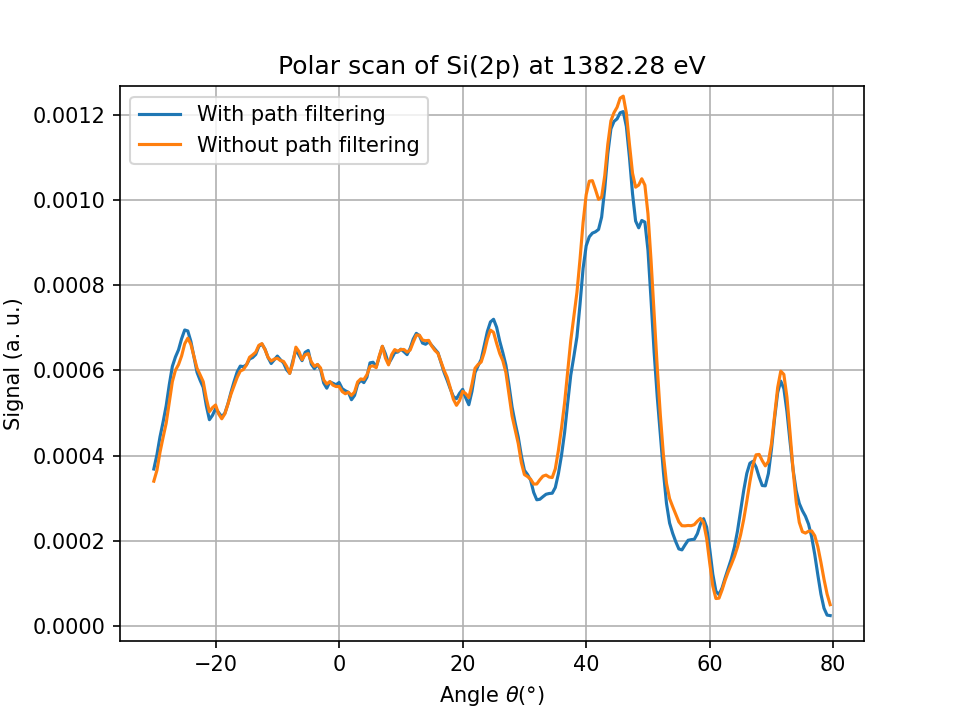
Fig. 18 Si(2p) polar scan (contribution of an emitter in the 4th plane with all 7 114 945 scattering paths taken into account (orange curve), and for only 1525 filtered paths (blue curve).#
 1# coding: utf8
 2
 3import numpy as np
 4from ase.build import bulk
 5
 6from msspec.calculator import MSSPEC, XRaySource
 7from msspec.iodata import Data
 8from msspec.utils import hemispherical_cluster, get_atom_index
 9
10
11# Create the cluster
12a = 5.43
13Si = bulk('Si', a=a, cubic=True)
14cluster = hemispherical_cluster(Si,
15                                diameter=30, planes=4,
16                                emitter_plane=3,
17                                shape = 'cylindrical',
18                                )
19for atom in cluster:
20    atom.set('mean_square_vibration', 0.006)
21    atom.set('mt_radius', 1.1)
22cluster.emitter = get_atom_index(cluster, 0, 0, 0)
23
24# Create a calculator and set parameters
25calc = MSSPEC(spectroscopy='PED', algorithm='expansion')
26
27calc.source_parameters.energy = XRaySource.AL_KALPHA
28calc.source_parameters.theta  = -54.7
29calc.source_parameters.phi    = 90
30calc.spectroscopy_parameters.final_state = 1
31
32calc.calculation_parameters.scattering_order = 3
33calc.tmatrix_parameters.tl_threshold = 1e-4
34calc.calculation_parameters.vibrational_damping = 'averaged_tl'
35calc.calculation_parameters.RA_cutoff = 2
36
37my_filters = ('forward_scattering', 'distance_cutoff')
38calc.calculation_parameters.path_filtering = my_filters
39calc.calculation_parameters.distance = 30
40calc.calculation_parameters.off_cone_events = 0
41[a.set('forward_angle', 40) for a in cluster]
42
43calc.set_atoms(cluster)
44
45# Compute and add previous data for comparison
46data = calc.get_theta_scan(level='2p',
47                            theta=np.arange(-30., 80., 0.5),
48                            phi=0,
49                            kinetic_energy=1382.28)
50no_filters = Data.load('path_filtering.hdf5')
51data[0].add_columns(**{'no_filters': no_filters[0].cross_section})
52view = data[0].views[0]
53view.select('theta', 'cross_section', index=0, legend="With path filtering")
54view.select('theta', 'no_filters', legend="Without path filtering")
55
56data.view()