Activity 9: Comparing simulation and experiment with R-factors

In order to extract precise crystallographic information from electronic spectroscopy, we need to compare MsSpec calculations with experimental results and adjust the modelling parameters to simulate the experiment as accurately as possible.

R-factors (reliability factors) are commonly used for this task. In the following example, we will see how MsSpec can extract the adsorption geometry of a molecule.

The unusual tilt of CO molecule on Fe(001)

The carbon monoxide molecule can be adsorbed onto a Fe(001) surface in the hollow site. It was experimentally demonstrated that the CO molecule is tilted by 55\(\pm\)2° in <100> azimuthal directions. The molecule is bonded to the Fe surface by the carbon atom and the adsorption height was estimated to be \(\sim\) 0.6 Å.

See also

based on this paper from R. S. Saiki et al. Phys. Rev. Lett. 63(3) p283-6 (1989)

We will try to reproduce the polar scan of the figure below of CO adsorbed in the hollow site of the Fe(001) surface with simple single scattering calculations with MsSpec and by using R-Factors to find the best adsorption geometry. We will use the simple cluster displayed on the left hand side of the figure.

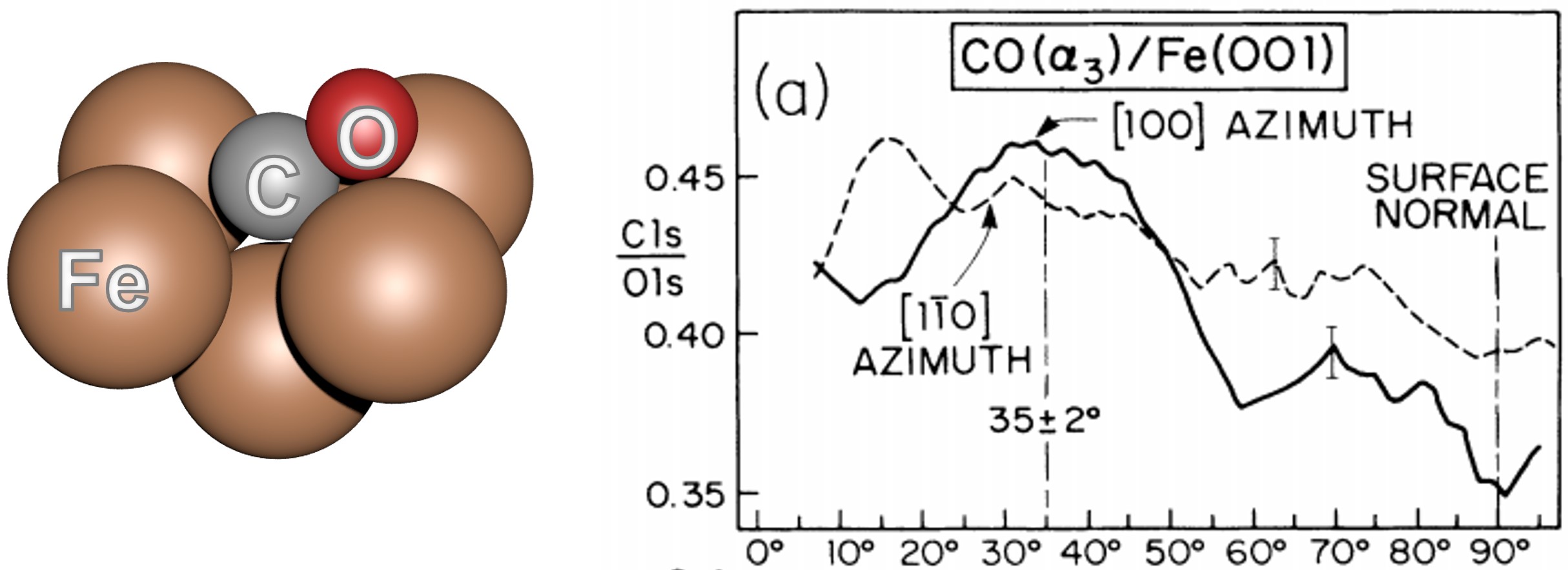
Fig. 24 Small cluster used for SSC calculations (left) and (right) Normalized polar scan of the C(1s) at 1202 eV for [100] and [1-10] azimths.

Quiz

Download this script and write the body of the function create_cluster. The function should return a small cluster of 5 Fe atoms with the CO molecule adsorbed like in figure Fig. 25 below. The function will accept 4 keyword arguments to control the adsorption geometry.

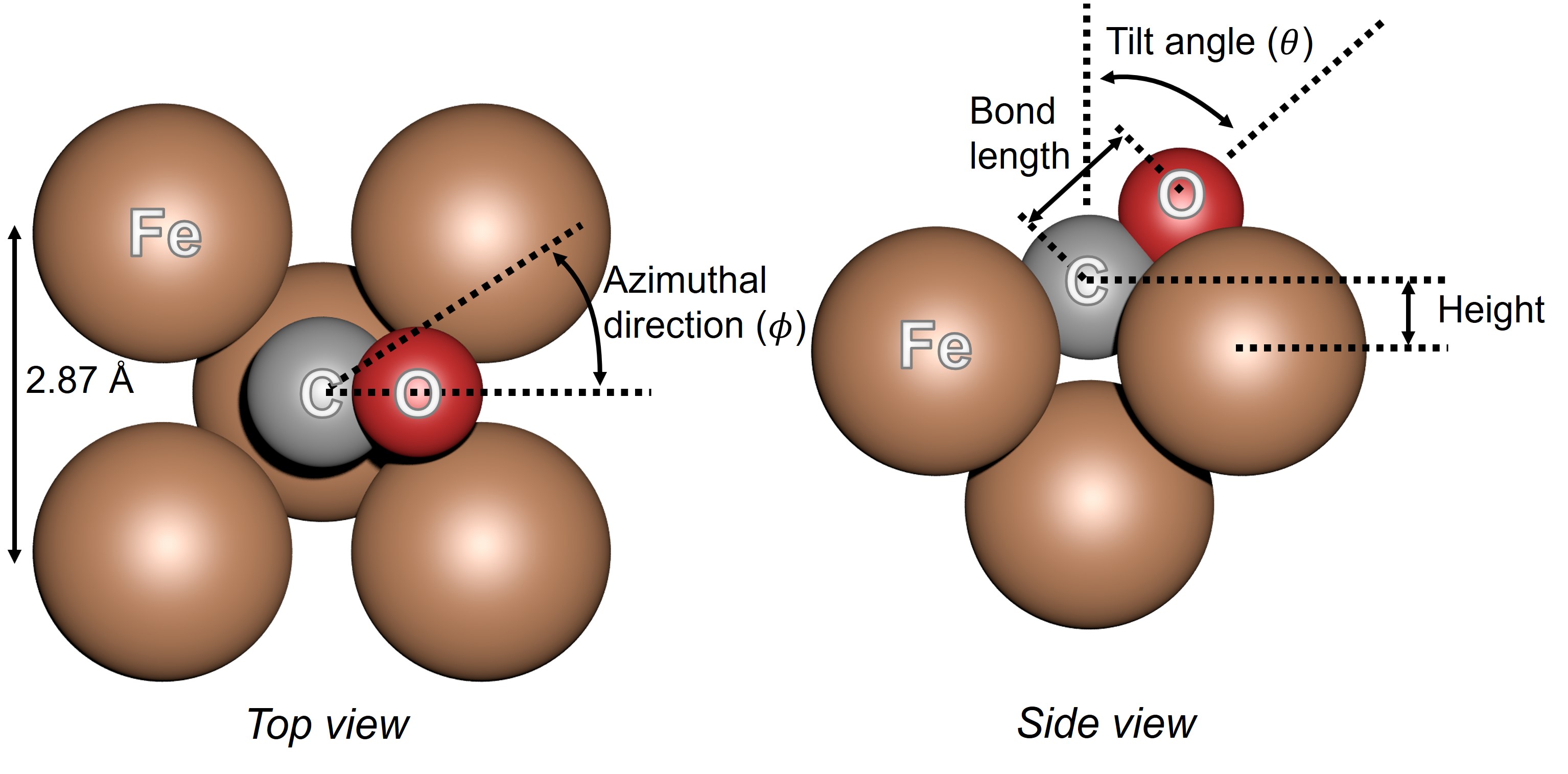
Fig. 25 Adsorption geometry of carbon monoxide on Fe(001).

Note

Remember to use the ase.build.bulk, the msspec.utils.hemispherical_cluster and the ase.build.add_adsorbate functions.

Here is the code of the create_cluster function

def create_cluster(height=1., theta=45, phi=0, bond_length=1.15):
    # Fill the body of this function. The 'cluster' object in built according to
    # values provided by the keyword arguments:
    # height (in angströms): the 'z' distance between the Fe surface and the C atom
    # theta and phi (in degrees): the polar and azimuthal orientation of the CP molecule
    #                             (theta=0° aligns the molecule withe the surface normal
    #                              phi=0° corresponds to the [100] direction of iron)
    # bond_length (in angströms): the C-O distance

    iron = bulk('Fe', cubic=True)
    cluster = hemispherical_cluster(iron, diameter=5, planes=2, emitter_plane=1)

    t = np.radians(theta)
    p = np.radians(phi)

    z = bond_length * np.cos(t)
    x = bond_length * np.sin(t) * np.cos(p)
    y = bond_length * np.sin(t) * np.sin(p)
    CO=Atoms('CO',positions=[(0,0,0),(x,y,z)])

    add_adsorbate(cluster,CO, height=height)

    # Keep those 2 lines at the end of your function
    # Store some information in the cluster object
    cluster.info.update(adsorbate={'theta': theta, 'phi': phi, 'height': height, 
                                   'bond_length': bond_length})

Now that the create_cluster function is done, look at the rest of the script. The next function is called compute_polar_scan and will obviously be used to compute the \(\theta\)-scan of the C1s for a given cluster geometry. Finally there is the Main part that is built in two sections:

1. A section containing nested for loops

2. A final section for R-Factor analysis

Quiz

1. Complete the nested for loops in section 1) in order to compute polar scans for CO molecule tilted from 45° to 60° with a 1° step and aligned either along the [100] direction of Fe, 30° from this direction or along [110]. The adsorption height is 0.6 Å and the bond length is 1.157 Å.

2. What is the best \((\theta, \phi)\) according to the R-Factor analysis

Here are the code of the nested for loops

###############################################################################
# Main part
###############################################################################
results    = [] # polar angles and calculated cross_sections will be appended
                # to this list after each 'compute_polar_scan' call
parameters = {'theta': [], 'phi': []} # and corresponding parameters will also
                                      # be stored in this dictionary

# 1) Run calculations for different geometries
for theta in np.arange(45, 60, 1):
    for phi in [0, 30, 45]:
        # Create the cluster
        cluster = create_cluster(theta=theta, phi=phi, height=0.6,
                                bond_length=1.157)
        # Compute
        data = compute_polar_scan(cluster)

        # Update lists of results and parameters
        results.append(data[-1].theta.copy())
        results.append(data[-1].cross_section.copy())
        parameters['theta'].append(theta)
        parameters['phi'].append(phi)

Runing the code gives the following result. The CO molecule belongs to the (100), (010), (-100), (0-10) planes of iron and is tilted by 55° from the surface normal (ie 35° from the surface itself).

Fig. 26 Best polar scan according to R-Factor analysis.

MsSpec uses 12 different R-Factors formula to compare the calculted curve to the experimental data. The set of parameters giving the best agreement according to the majority of those 12 R-factors is assumed to be the best solution. Here are the R-factors formula used in MsSpec

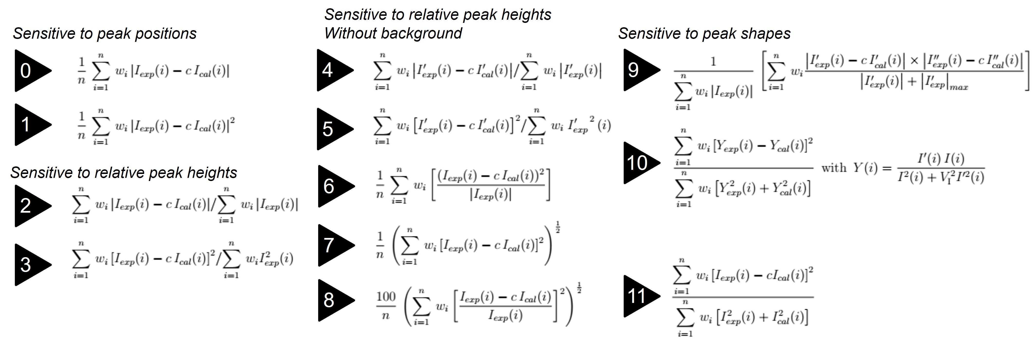
Fig. 27 The 12 R-Factors used in MsSpec. The Pendry’s R-Factor is n° ??

Quiz

How many R-Factors do agree that \((\theta,\phi)=(55,0)\) gives the best agreement ?

6 R-factors out of 12 do agree that variable set n°30 gives the best agreement. The set n°30 corresponds to \(\theta=55°\) and \(\phi=0°\).

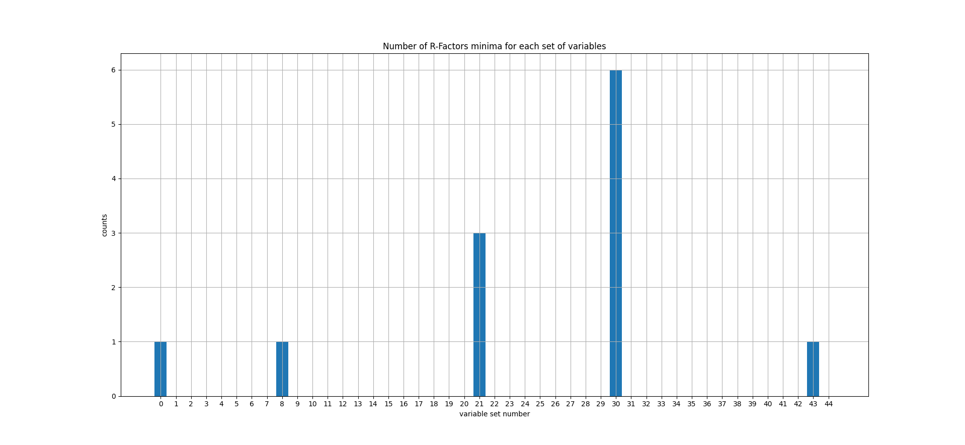
Fig. 28 The number of R-Factors for which the parameter set (in abscissa) gives the best agreement.