Activity 1: Getting started#
MsSpec is a Fortran code with two components: Phagen (Written by R. Natoli) and Spec (written by D. Sébilleau). Phagen computes the phase shifts of the electronic wave propagating in the matter on a spherical harmonics basis. Spec uses those phase shifts to compute the multiple scattering process and simulate the intensity of different electronic spectroscopies.
In the most recent version of MsSpec, the program is interfaced with python (https://msspec.cnrs.fr/), allowing for much more flexibility and interplay with other simulation techniques.
Building atomic systems#
MsSpec works in the cluster approach. Building such a cluster for a calculation is a fundamental step. We use the python Atomic Simulation Environment (ASE) for this.
ASE is a set of tools and Python modules for setting up, manipulating, running, visualizing and analyzing atomistic simulations. Building atomic systems, structures… is pretty straightforward:
# To build a molecule with ASE
from ase.build import molecule
# To view
from ase.visualize import view

# Create a water molecule
water = molecule('H2O')
# Display it
view(water)
Barebone script for MsSpec#
MsSpec can simulate different electronic spectroscopies like PED, AED, LEED, EXAFS, APECS and more will be included in the forthcoming version. However, it is really well-suited for PhotoElectron Diffraction simulation, and the python interface is only fully available for it at the moment. Since PED covers all the MsSpec features and concepts, we will focus on this technique.
There are typically 3 steps to follow to get a result with MsSpec:
Create a cluster
Create an ASE calculator
Run the simulation
PED polar scan for Cu(001)#
1from ase.io import read
2from msspec.calculator import MSSPEC
3
4
5cluster = read('copper.cif')
6# view the cluster
7cluster.edit()
8
 9# The "emitter" atom is located in the middle of the 3rd plane
10cluster.emitter = 10
11
12# Create a "calculator"
13calc = MSSPEC(spectroscopy='PED', algorithm='inversion')
14calc.set_atoms(cluster)
15
16data = calc.get_theta_scan(level='2p3/2')
17
18# Plot the result with the interactive GUI
19data.view()
20
21# Or plot using matplotlib directly
22from matplotlib import pyplot as plt
23data[0].views[0].plot()
24plt.show()
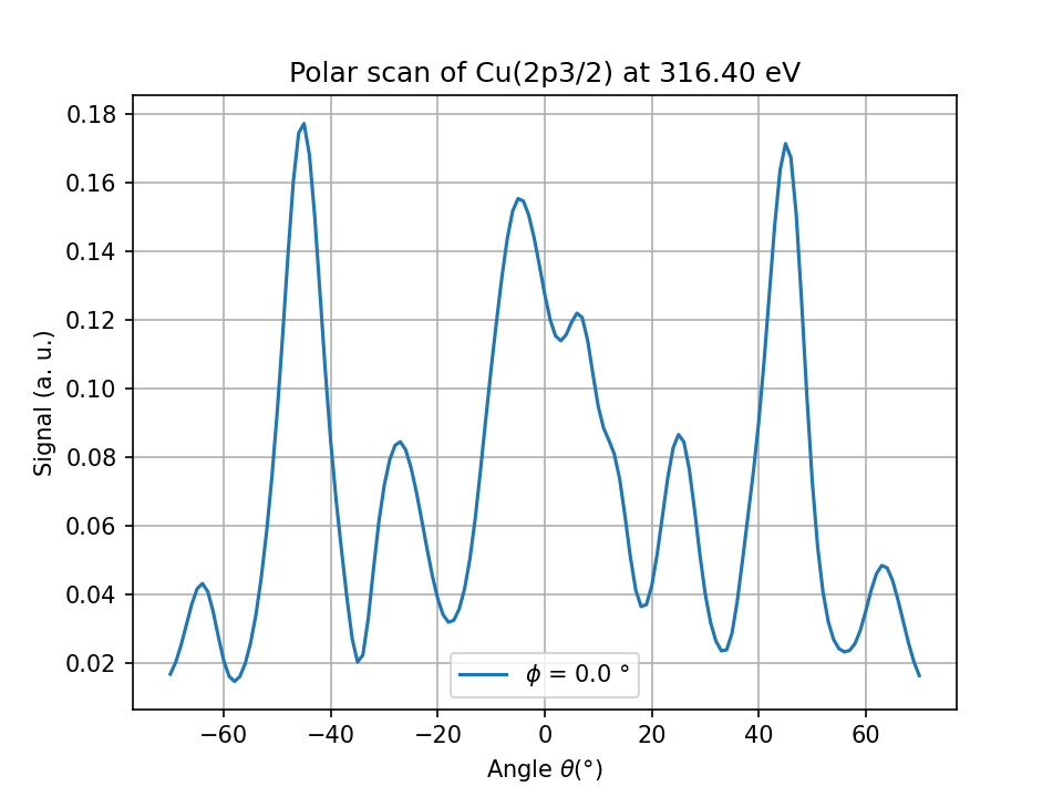
Fig. 1 Cu(2p) polar scan for the copper cluster above#
Shaping a cluster#
Based on the previous *.cif file, create a new cluster without the deepest plane and run the same calculation for the same emitter
Note
As the cluster will contain fewer atoms, the emitter index will be different
What do you conclude ?
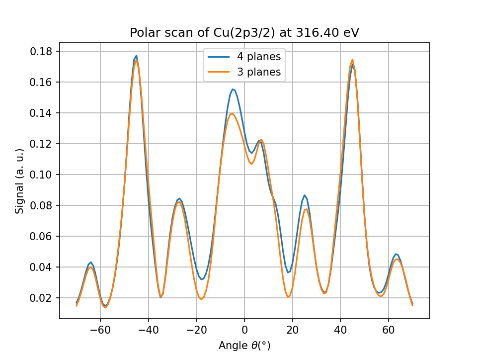
Fig. 2 Comparison between 4 and 3 planes for an emitter in the 3rd plane.#
Not all atoms contribute equally to the total signal. Some of them can be removed to save computation time and memory.
The number of atoms used for the calculation greatly impact the calculation time and memory. Most of the time, a cluster is shaped as an hemisphere to minimize the number of atoms to take into account
from msspec.calculator import MSSPEC
from msspec.utils import hemispherical_cluster, get_atom_index
from ase.build import bulk
from ase.visualize import view

copper = bulk('Cu', cubic=True)
cluster = hemispherical_cluster(copper, planes=3, emitter_plane=2)
cluster.emitter = get_atom_index(cluster, 0,0,0)

view(cluster)
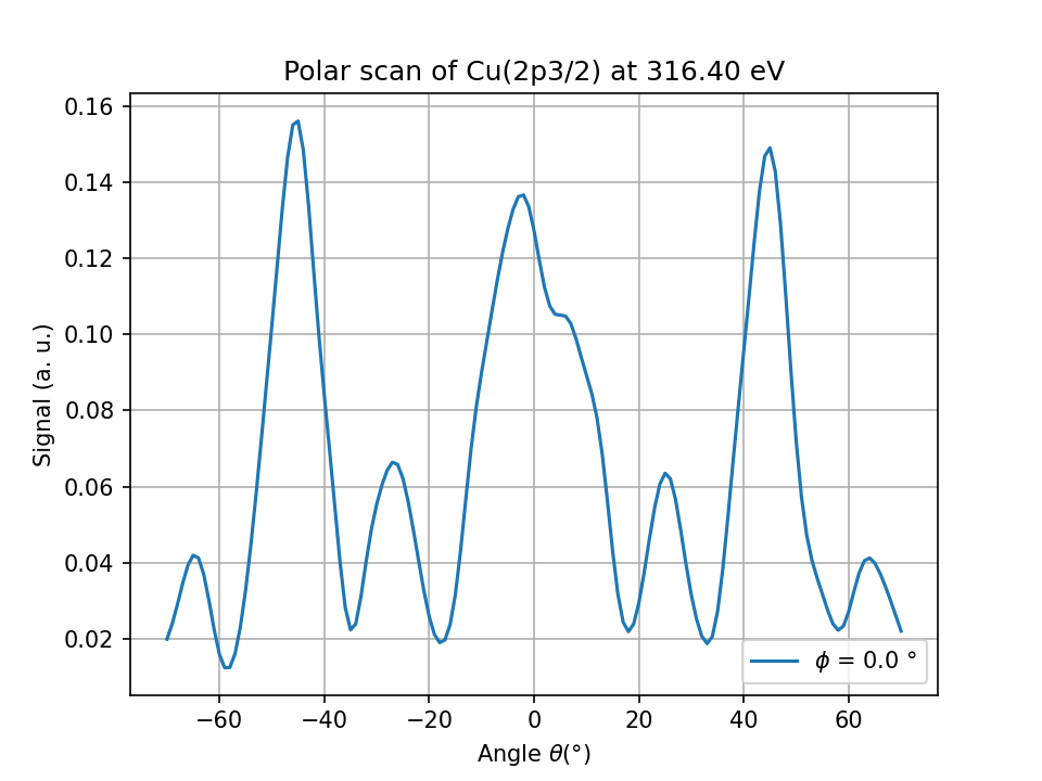
Fig. 3 Cu(2p) polar scan for the hemispherical cluster.#